Getting started with Pema
2/11/2021
Basic examples of how to use pema easily
below we will explain - how to run pema - What types of outputs we can get to match peaks and events
Starting a context
Just as in wfsim or straxen we need a context. In this example, we use a context from straxen but pema also has it’s own context if you want to have some more expert experience of of the fine details of the package
[1]:
import pema
import straxen
import wfsim
import pandas as pd
import logging
import matplotlib.pyplot as plt
import numpy as np

# WFSim can be quite verboose, let's increase the loggers verbosity
logging.getLogger().setLevel(logging.ERROR)
[2]:
straxen.print_versions('strax straxen wfsim pema'.split())
Working on dali013.rcc.local with the following versions and installation paths:
python  v3.8.5  (default, Sep  4 2020, 07:30:14) [GCC 7.3.0]
strax   v1.1.2  /home/angevaare/software/strax/strax    git branch:master | 9b79ca7
straxen v1.1.3  /home/angevaare/software/straxen/straxen        git branch:master | e7d3d02
wfsim   v0.5.12 /home/angevaare/software/wfsim/wfsim    git branch:master | 0d74d97
pema    v0.3.5  /home/angevaare/software/pema/pema      git branch:master | 5b54328
[3]:
run_id = '026000'
st = wfsim.contexts.xenonnt_simulation(cmt_run_id_sim=run_id)
Write some instruction file for WFSim
This is just to make a CSV file with ~100 events so that we don’t simulate for a long time
[4]:
instructions = dict(
    event_rate=50,
    chunk_size=1,
    n_chunk=2,
    tpc_radius=straxen.tpc_r,
    tpc_length=straxen.tpc_z,
    drift_field=10,
    energy_range=[1, 10],  # keV
    nest_inst_types=wfsim.NestId.ER,
)
instructions_path = './inst.csv'
[ ]:
# Write these instructions to the instructions_path
pema.inst_to_csv(
            instructions_path,
            get_inst_from=pema.rand_instructions,
            **instructions)
if we now look at the instructions, we see that the instructions are in the format WFSim needs
[6]:
pd.read_csv(instructions_path).head(5)
[6]:
| event_number | type | time | x | y | z | amp | recoil | e_dep | g4id | vol_id | local_field | n_excitons | |
|---|---|---|---|---|---|---|---|---|---|---|---|---|---|
| 0 | 0 | 1 | 10000000 | 0.213643 | -50.968160 | -66.82086 | 570 | 7 | 8.762822 | -1 | -1 | 10.0 | 46 |
| 1 | 0 | 2 | 10000000 | 0.213643 | -50.968160 | -66.82086 | 78 | 7 | 8.762822 | -1 | -1 | 10.0 | 0 |
| 2 | 0 | 1 | 30000000 | 18.600367 | 37.217890 | -54.83090 | 263 | 8 | 5.303098 | -1 | -1 | 10.0 | 18 |
| 3 | 0 | 2 | 30000000 | 18.600367 | 37.217890 | -54.83090 | 121 | 8 | 5.303098 | -1 | -1 | 10.0 | 0 |
| 4 | 0 | 1 | 50000000 | -20.259249 | -10.839966 | -92.56312 | 1001 | 11 | 7.181198 | -1 | -1 | 10.0 | 72 |
Running wfsim
Nothing fancy, just make some data
[ ]:
st.set_config({'fax_file': instructions_path})
st.make('026000', 'raw_records')
Why we need pema?
So after running the simulator, we can now have a look at the truth data and the reconstructed data. You will notice that these are not very trivial to match, the size etc. of the data is different making it hard to compare directly
[8]:
st.get_df(run_id, 'truth').head(5)
[8]:
| event_number | type | time | x | y | z | amp | recoil | e_dep | g4id | ... | t_first_photon | t_last_photon | t_mean_photon | t_sigma_photon | x_mean_electron | y_mean_electron | t_first_electron | t_last_electron | t_mean_electron | t_sigma_electron | |
|---|---|---|---|---|---|---|---|---|---|---|---|---|---|---|---|---|---|---|---|---|---|
| 0 | 0 | 1 | 10000037 | 0.213643 | -50.968159 | -66.820862 | 570 | 7 | 8.762822 | -1 | ... | 10000037.0 | 10000310.0 | 1.000010e+07 | 51.623532 | NaN | NaN | NaN | NaN | NaN | NaN |
| 1 | 0 | 2 | 10982323 | 0.213643 | -50.968159 | -66.820862 | 78 | 7 | 8.762822 | -1 | ... | 10982323.0 | 10999426.0 | 1.099032e+07 | 3323.948834 | NaN | NaN | 10982770.0 | 10998267.0 | 1.099008e+07 | 3305.199797 |
| 2 | 0 | 1 | 30000025 | 18.600367 | 37.217892 | -54.830898 | 263 | 8 | 5.303098 | -1 | ... | 30000025.0 | 30000280.0 | 3.000010e+07 | 63.100088 | NaN | NaN | NaN | NaN | NaN | NaN |
| 3 | 0 | 2 | 30805117 | 18.600367 | 37.217892 | -54.830898 | 121 | 8 | 5.303098 | -1 | ... | 30805117.0 | 30821781.0 | 3.081305e+07 | 3013.418322 | NaN | NaN | 30805767.0 | 30820812.0 | 3.081293e+07 | 3084.207357 |
| 4 | 0 | 1 | 50000030 | -20.259249 | -10.839966 | -92.563118 | 1001 | 11 | 7.181198 | -1 | ... | 50000030.0 | 50000354.0 | 5.000010e+07 | 54.821558 | NaN | NaN | NaN | NaN | NaN | NaN |
5 rows × 37 columns
[9]:
st.get_df(run_id, 'peak_basics').head(5)
[9]:
| time | endtime | center_time | area | n_channels | max_pmt | max_pmt_area | n_saturated_channels | range_50p_area | range_90p_area | area_fraction_top | length | dt | rise_time | tight_coincidence | tight_coincidence_channel | type | |
|---|---|---|---|---|---|---|---|---|---|---|---|---|---|---|---|---|---|
| 0 | 10000020 | 10000550 | 10000143 | 90.596260 | 56 | 253 | 4.146482 | 0 | 79.069336 | 223.482574 | 0.190108 | 53 | 10 | 48.225266 | 49 | 48 | 1 |
| 1 | 10982310 | 10999590 | 10990290 | 2977.601807 | 407 | 30 | 328.906281 | 0 | 4870.469238 | 11093.649414 | 0.705678 | 192 | 90 | 4130.819336 | 27 | 23 | 2 |
| 2 | 30000010 | 30000520 | 30000141 | 38.071171 | 26 | 460 | 3.673802 | 0 | 90.643417 | 243.026779 | 0.138739 | 51 | 10 | 62.914806 | 15 | 14 | 1 |
| 3 | 30805100 | 30821930 | 30813033 | 4511.850586 | 451 | 219 | 485.288208 | 0 | 4094.857422 | 9902.229492 | 0.680726 | 187 | 90 | 3647.358887 | 63 | 60 | 2 |
| 4 | 50000010 | 50000590 | 50000151 | 135.912338 | 88 | 325 | 5.080719 | 0 | 83.577980 | 241.828125 | 0.242879 | 58 | 10 | 56.064529 | 84 | 80 | 1 |
Using pema we can easily match events and peaks
First, let’s register pema to the context
[10]:
st.register_all(pema.match_plugins)
[11]:
df = st.get_df(run_id, 'match_acceptance_extended')
df.head(10)
[11]:
| time | endtime | is_found | acceptance_fraction | rec_bias | event_number | type | x | y | z | ... | t_sigma_photon | x_mean_electron | y_mean_electron | t_first_electron | t_last_electron | t_mean_electron | t_sigma_electron | id | outcome | matched_to | |
|---|---|---|---|---|---|---|---|---|---|---|---|---|---|---|---|---|---|---|---|---|---|
| 0 | 10000037 | 10000310 | True | 1.0 | 1.352183 | 0 | 1 | 0.213643 | -50.968159 | -66.820862 | ... | 51.623532 | NaN | NaN | NaN | NaN | NaN | NaN | 0 | found | 0 |
| 1 | 10982323 | 10999426 | True | 1.0 | 1.250043 | 0 | 2 | 0.213643 | -50.968159 | -66.820862 | ... | 3323.948834 | NaN | NaN | 10982770.0 | 10998267.0 | 1.099008e+07 | 3305.199797 | 1 | found | 1 |
| 2 | 30000025 | 30000280 | True | 1.0 | 1.189724 | 0 | 1 | 18.600367 | 37.217892 | -54.830898 | ... | 63.100088 | NaN | NaN | NaN | NaN | NaN | NaN | 2 | found | 2 |
| 3 | 30805117 | 30821781 | True | 1.0 | 1.232409 | 0 | 2 | 18.600367 | 37.217892 | -54.830898 | ... | 3013.418322 | NaN | NaN | 30805767.0 | 30820812.0 | 3.081293e+07 | 3084.207357 | 3 | found | 3 |
| 4 | 50000030 | 50000354 | True | 1.0 | 1.192213 | 0 | 1 | -20.259249 | -10.839966 | -92.563118 | ... | 54.821558 | NaN | NaN | NaN | NaN | NaN | NaN | 4 | found | 4 |
| 5 | 51358856 | 51381325 | True | 1.0 | 1.255800 | 0 | 2 | -20.259249 | -10.839966 | -92.563118 | ... | 3764.153809 | NaN | NaN | 51359296.0 | 51380713.0 | 5.137001e+07 | 3786.530135 | 5 | found | 5 |
| 6 | 70000016 | 70000382 | True | 1.0 | 1.187851 | 0 | 1 | -47.578213 | 0.588989 | -137.323624 | ... | 83.635968 | NaN | NaN | NaN | NaN | NaN | NaN | 6 | found | 6 |
| 7 | 72020959 | 72040738 | True | 1.0 | 1.205682 | 0 | 2 | -47.578213 | 0.588989 | -137.323624 | ... | 3683.165652 | NaN | NaN | 72021418.0 | 72040323.0 | 7.203114e+07 | 3681.208360 | 7 | found | 7 |
| 8 | 90000036 | 90000390 | True | 1.0 | 1.297663 | 0 | 1 | -55.136837 | -7.310527 | -145.262833 | ... | 66.397138 | NaN | NaN | NaN | NaN | NaN | NaN | 8 | found | 8 |
| 9 | 92137377 | 92161298 | True | 1.0 | 1.254083 | 0 | 2 | -55.136837 | -7.310527 | -145.262833 | ... | 4783.696419 | NaN | NaN | 92137889.0 | 92160617.0 | 9.214823e+07 | 4747.782437 | 9 | found | 9 |
10 rows × 43 columns
We see that we have many more colums to choose from, like is_found, rec_bias, matched_to etc. You can have a look at all the fields here:
[12]:
st.data_info('truth_extended')
[12]:
| Field name | Data type | Comment | |
|---|---|---|---|
| 0 | time | int64 | Start time since unix epoch [ns] |
| 1 | endtime | int64 | Exclusive end time since unix epoch [ns] |
| 2 | is_found | bool | Is the peak tagged "found" in the reconstructe... |
| 3 | acceptance_fraction | float64 | Acceptance of the peak can be negative for pen... |
| 4 | rec_bias | float64 | Reconstruction bias 1 is perfect, 0.1 means in... |
| 5 | event_number | int32 | Waveform simulator event number. |
| 6 | type | int8 | Quanta type (S1 photons or S2 electrons) |
| 7 | x | float32 | X position of the cluster [cm] |
| 8 | y | float32 | Y position of the cluster [cm] |
| 9 | z | float32 | Z position of the cluster [cm] |
| 10 | amp | int32 | Number of quanta |
| 11 | recoil | int8 | Recoil type of interaction. |
| 12 | e_dep | float32 | Energy deposit of interaction |
| 13 | g4id | int32 | Eventid like in geant4 output rootfile |
| 14 | vol_id | int32 | Volume id giving the detector subvolume |
| 15 | local_field | float64 | Local field [ V / cm ] |
| 16 | n_excitons | int32 | Number of excitons |
| 17 | n_electron | int32 | Number of simulated electrons |
| 18 | n_photon | int32 | Number of photons reaching PMT |
| 19 | n_pe | int32 | Number of photons + dpe passing |
| 20 | n_photon_trigger | int32 | Number of photons passing trigger |
| 21 | n_pe_trigger | int32 | Number of photons + dpe passing trigger |
| 22 | raw_area | float64 | Raw area in pe |
| 23 | raw_area_trigger | float64 | Raw area in pe passing trigger |
| 24 | n_photon_bottom | int32 | Number of photons reaching PMT (bottom) |
| 25 | n_pe_bottom | int32 | Number of photons + dpe passing (bottom) |
| 26 | n_photon_trigger_bottom | int32 | Number of photons passing trigger (bottom) |
| 27 | n_pe_trigger_bottom | int32 | Number of photons + dpe passing trigger (bottom) |
| 28 | raw_area_bottom | float64 | Raw area in pe (bottom) |
| 29 | raw_area_trigger_bottom | float64 | Raw area in pe passing trigger (bottom) |
| 30 | t_first_photon | float64 | Arrival time of the first photon [ns] |
| 31 | t_last_photon | float64 | Arrival time of the last photon [ns] |
| 32 | t_mean_photon | float64 | Mean time of the photons [ns] |
| 33 | t_sigma_photon | float64 | Standard deviation of photon arrival times [ns] |
| 34 | x_mean_electron | float32 | X field-distorted mean position of the electro... |
| 35 | y_mean_electron | float32 | Y field-distorted mean position of the electro... |
| 36 | t_first_electron | float64 | Arrival time of the first electron [ns] |
| 37 | t_last_electron | float64 | Arrival time of the last electron [ns] |
| 38 | t_mean_electron | float64 | Mean time of the electrons [ns] |
| 39 | t_sigma_electron | float64 | Standard deviation of electron arrival times [ns] |
| 40 | id | int64 | Id of element in truth |
| 41 | outcome | <U32 | Outcome of matching to peaks |
| 42 | matched_to | int64 | Id of matching element in peaks |
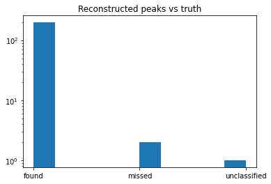
For example, we can now look at the outcome of the matching. We look at what each of the peaks in truth results to in peaks in the data. For example, one instruction can be split into multiple peaks (split) or completely missed by the reconstruction software (missed)
[13]:
plt.hist(df['outcome'])
plt.yscale('log')
plt.title('Reconstructed peaks vs truth')
[13]:
Text(0.5, 1.0, 'Reconstructed peaks vs truth')
For events, we can do something similar
[14]:
st.data_info('truth_events')
[14]:
| Field name | Data type | Comment | |
|---|---|---|---|
| 0 | time | int64 | Start time since unix epoch [ns] |
| 1 | endtime | int64 | Exclusive end time since unix epoch [ns] |
| 2 | start_match | int64 | First event number in event datatype within th... |
| 3 | end_match | int64 | Last (inclusive!) event number in event dataty... |
| 4 | outcome | <U32 | Outcome of matching to events |
| 5 | truth_number | int64 | Truth event number |
[15]:
st.show_config('truth_events')
[15]:
| option | default | current | applies_to | help | |
|---|---|---|---|---|---|
| 0 | penalty_s2_by | ((misid_as_s1, -1.0), (split_and_misid, -1.0)) | <OMITTED> | (match_acceptance,) | Add a penalty to the acceptance fraction if th... |
| 1 | min_s2_bias_rec | 0.85 | <OMITTED> | (match_acceptance,) | If the S2 fraction is greater or equal than th... |
| 2 | detector | XENONnT | XENONnT | (raw_records, raw_records_he, raw_records_aqmo... | |
| 3 | event_rate | 1000 | <OMITTED> | (raw_records, raw_records_he, raw_records_aqmo... | Average number of events per second |
| 4 | chunk_size | 100 | <OMITTED> | (raw_records, raw_records_he, raw_records_aqmo... | Duration of each chunk in seconds |
| ... | ... | ... | ... | ... | ... |
| 71 | max_drift_length | 148.6515 | <OMITTED> | (events,) | Total length of the TPC from the bottom of gat... |
| 72 | exclude_s1_as_triggering_peaks | True | <OMITTED> | (events,) | If true exclude S1s as triggering peaks. |
| 73 | min_area_fraction | 0.5 | <OMITTED> | (peak_proximity,) | The area of competing peaks must be at least t... |
| 74 | nearby_window | 10000000 | <OMITTED> | (peak_proximity,) | Peaks starting within this time window (on eit... |
| 75 | peak_max_proximity_time | 100000000 | <OMITTED> | (peak_proximity,) | Maximum value for proximity values such as t_t... |
76 rows × 5 columns
In fact we see that we did not do this very intelligently, the random instructions just specified 2 events, each with broad spacing and ~50 peaks/event. As such these two “events” are split into 50 events
[16]:
df_truth_events = st.get_df(run_id, 'truth_events')
df_truth_events.head()
[16]:
| time | endtime | start_match | end_match | outcome | truth_number | |
|---|---|---|---|---|---|---|
| 0 | 10000037 | 990930702 | 0 | 49 | split | 0 |
| 1 | 1010000044 | 1990220979 | 50 | 103 | split | 1 |
Now you might want to open each of the events in according to a grouping one had in the truth file. Let’s for example open event 0 from the truth file
[17]:
events = st.get_df(run_id, ('events', 'event_basics'))
[18]:
truth_selection = df_truth_events['truth_number'] == 0
[19]:
event_selection = [
    ((ev['start_match'] <= events['event_number']) &
     (events['event_number'] <= ev['end_match']))
    for i, ev in
    df_truth_events[truth_selection].iterrows()
]
event_selection = np.any(event_selection, axis=0)
[20]:
events[event_selection].head()
[20]:
| time | endtime | n_peaks | drift_time | event_number | s1_index | alt_s1_index | s1_time | alt_s1_time | s1_center_time | ... | alt_s2_x_cnn | alt_s2_y_cnn | s2_x_gcn | s2_y_gcn | alt_s2_x_gcn | alt_s2_y_gcn | s2_x_mlp | s2_y_mlp | alt_s2_x_mlp | alt_s2_y_mlp | |
|---|---|---|---|---|---|---|---|---|---|---|---|---|---|---|---|---|---|---|---|---|---|
| 0 | 9900000 | 11249590 | 2 | 990147.0 | 0 | 0 | -1 | 10000020 | -1 | 10000143 | ... | NaN | NaN | 0.367014 | -50.836010 | NaN | NaN | 0.301356 | -51.021992 | NaN | NaN |
| 1 | 28359362 | 31071930 | 2 | 812892.0 | 1 | 0 | -1 | 30000010 | -1 | 30000141 | ... | NaN | NaN | 18.742008 | 37.128674 | NaN | NaN | 18.763103 | 37.098461 | NaN | NaN |
| 2 | 48913102 | 51631400 | 2 | 1369899.0 | 2 | 0 | -1 | 50000010 | -1 | 50000151 | ... | NaN | NaN | -19.878204 | -10.981473 | NaN | NaN | -19.933523 | -10.953871 | NaN | NaN |
| 3 | 69575202 | 72290960 | 2 | 2030929.0 | 3 | 0 | -1 | 70000000 | -1 | 70000165 | ... | NaN | NaN | -47.723724 | 0.776461 | NaN | NaN | -47.679546 | 0.850672 | NaN | NaN |
| 4 | 89691622 | 92411410 | 2 | 2148194.0 | 4 | 0 | -1 | 90000020 | -1 | 90000172 | ... | NaN | NaN | -55.278717 | -7.305344 | NaN | NaN | -55.405975 | -7.268640 | NaN | NaN |
5 rows × 91 columns